Stock

Patrick G. Eddington

Two actions this week highlight the Biden administration’s approach to surveillance issues implicating the constitutional rights of Americans.

The first is an executive order (EO) issued on February 28, 2024, that, in relevant part, directs the attorney general to issue regulations

… that prohibit or otherwise restrict United States persons from engaging in any acquisition, holding, use, transfer, transportation, or exportation of, or dealing in, any property in which a foreign country or national thereof has any interest (transaction), where the transaction:

(i) involves bulk sensitive personal data or United States Government‐​related data, as further defined by regulations issued by the Attorney General pursuant to this section;

(ii) is a member of a class of transactions that has been determined by the Attorney General, in regulations issued by the Attorney General pursuant to this section, to pose an unacceptable risk to the national security of the United States because the transactions may enable countries of concern or covered persons to access bulk sensitive personal data or United States Government‐​related data in a manner that contributes to the national emergency described in this order;

It’s safe to say that this is the next step in the “ban TikTok” movement that’s become one of the few bipartisan hobby horses in Washington in recent years. It’s also a perfect example of political hypocrisy in that President Biden’s presidential campaign established its own TikTok account a little over two week’s ago, with CNBC reporting that “Biden campaign advisors told NBC News the TikTok account is part of an effort to meet voters where they are.”

This EO is noteworthy in that it argues that “bulk sensitive personal data” flows to countries like China are a national security threat while providing no evidence that such data flows have, in fact, led to compromises of classified information, systems, or programs.

And then there’s the hypocrisy of the EO in terms of who it targets versus who is exempt from it.

Biden’s EO does nothing to stop the FBI, the Drug Enforcement Administration, the Bureau of Alcohol, Tobacco, Firearms and Explosives, Homeland Security Investigations, US Immigration and Customs Enforcement, US Customs and Border Protection, or any other federal law enforcement agency from obtaining exactly the same kind of data broker–derived personal information on Americans that it seeks to keep out of the hands of China, Russia, etc. And it is those very agencies and their commercial data acquisition practices that led the House Judiciary Committee in December 2023 to vote 35–2 in support of the Protect Liberty and End Warrantless Surveillance Act (PLEWSA), which would, among other things, amend the Foreign Intelligence Surveillance Act (FISA) to mandate a warrant to obtain such data.

And the strong bipartisan support for PLEWSA brings me to the other Biden administration surveillance‐​related action this week: an attempt to get FISA renewed without congressional approval.

The same day the Biden EO on data flow bans or restrictions via foreign entities was announced, The New York Times reported:

The law had been set to expire in December, but Congress voted to extend it until April 19 to give itself more time to debate proposed changes. Lawmakers have yet to reach a consensus, and this month, a plan to hold a floor vote on the matter collapsed in the Republican‐​controlled House before a two‐​week recess.

The legislative paralysis has brought the calendar to the moment when the Justice Department and the Office of the Director of National Intelligence each year normally ask the Foreign Intelligence Surveillance Court to issue new certifications allowing the program to operate.

The law essentially requires the executive branch to ask the court to renew the certifications at least a month before they lapse to ensure there is no gap in coverage. The current orders governing the program expire on April 12, and officials have said they build in another week to give communications companies time to adjust their systems to any changes.

The law also says the program can keep going for the duration of annual orders from the court—even if the underlying statute expires in the meantime.

The New York Times claims that the administration is seeking an extension of the existing FISA Section 702 orders through April 19, 2025.

In theory, this kind of legal play by the Biden administration would only apply to persons or entities currently targeted under the program. But what about new alleged threats discovered after any Foreign Intelligence Surveillance Court approval of an extension of 702 authority through April 2025?

Based on a Clinton administration–era precedent, the next president could simply direct the National Security Agency or the Central Intelligence Agency (CIA) to carry out new electronic surveillance targeting under EO 12333.

We know about this precedent thanks to an ongoing Cato Freedom of Information Act lawsuit against the Privacy and Civil Liberties Oversight Board and the revelation of a CIA electronic surveillance program under EO 12333 between at least 1995 and 2000.

If a president were to designate such surveillance a covert action, it could be carried out without the House or Senate Judiciary Committees (the normal committees of jurisdiction for FISA) being informed; notification would only go to the House and Senate Intelligence Committees and the senior‐​most leadership of the House and Senate—which historically have been very pro‐​surveillance regardless of party affiliation.

It may also be that the Biden administration has leaked this potential FISA congressional end‐​run ploy as a means of putting fresh pressure on House Speaker Mike Johnson (R‑LA) to once again bring a FISA Section 702 renewal bill to the House floor before the current April 19, 2024, FISA Section 702 expiration date.

Either way, the fight over efforts to protect Americans from unwarranted or even illegal surveillance by their own government is only intensifying.

Romina Boccia and Dominik Lett

Legislators and the public tend to underestimate the fiscal costs of emergency spending. Emergency supplemental bills, such as the Ukraine‐​Israel foreign aid package, are often billed as one‐​time, temporary costs. This framing obscures the tens of billions of dollars in interest costs generated by new deficit spending. It also ignores Congress’ increasing reliance on emergency spending to circumvent budget controls.

Without commonsense reforms, Congress is likely to continue to abuse emergency spending at the expense of the nation’s fiscal health.

The Senate recently passed a multi‐​billion‐​dollar foreign aid bill that provides emergency funding for Ukraine, Israel, and other objectives. Some House representatives have countered with a trimmed funding package. Any foreign aid package will face an uphill battle due to impending budget deadlines, skepticism over the necessity of additional funding, and demands that foreign aid spending be tied to tighter southern border control.

What these conversations miss is that the cost of these bills extends far beyond the perceived one‐ or two‐​year funding timeline. In a high‐​interest rate environment, the long‐​term costs of new emergency deficit spending are many billions higher than legislators or the public might think.

The US faces a mounting fiscal challenge, primarily driven by automatic entitlement spending that most legislators refuse to touch. Casual emergency deficit spending is symptomatic of the bigger problem: Washington remains mired in myopic budget thinking. Congress should adopt prudent, forward‐​thinking budget reforms, such as more accurate legislative cost‐​scoring and emergency spending controls.

Short‐​term Interest Costs of “Temporary” Emergency Spending

The Senate’s stated foreign aid bill cost is $95 billion. We can use a Congressional Budget Office (CBO) tool to estimate the debt‐​service costs of new deficit spending based on CBO’s interest rate projections. Assuming all $95 billion is spent in fiscal year (FY) 2024, the debt‐​service costs over the next 10 years are $41 billion. In total, the bill will really cost $136 billion over the next decade.

The stated cost of the trimmed House’s foreign aid package is $66 billion. Under the same assumptions, debt service costs over the next 10 years are $28 billion. That’s $95 billion over the next 10 years—the same as the advertised cost of the Senate package.

Emergency spending, such as the two foreign aid packages outlined above, is almost always deficit spending and does not follow normal budget protocols. As a result, emergency deficit spending tends to increase interest costs over the long term. According to CBO projections, interest costs are projected to grow by 87 percent in the next 10 years. In FY 2024, interest costs will exceed all defense spending.

If legislators engage in more casual deficit spending, they will directly contribute to the debt problem now by digging the fiscal hole even deeper. For decades, Washington enjoyed cheap borrowing thanks to low‐​interest rates. Now, thanks to excessive pandemic emergency spending, the situation has radically changed.

Despite a fundamentally different interest rate dynamic, some lawmakers appear intent on continuing deficit spending as usual. Continuing prior Congresses’ spending‐​prone behaviors would be brash and place a significant burden on current and future taxpayers who are on the hook for elevated federal debt.

Emergency Budget Reform Is Commonsense Fiscal Policy

These two reforms would help to address irresponsible emergency spending. First, legislators should require CBO to include projected interest costs in legislative cost estimates. This would more accurately reflect the cost of new deficit spending while also reducing reliance on costly gimmicky budget tricks. One such gimmick, called “spend now, save later,” involves offsetting new spending with uncertain, future spending cuts or revenue increases. Since these savings are delayed until the end of the 10‐​year budget window, legislators do not fully offset the impact of new deficit spending and associated interest costs.

Second, legislators should implement an offsetting mechanism to track and pay for emergency spending including interest costs. Such a budgeting mechanism would incentivize long‐​term fiscal planning while granting legislators the flexibility to respond to crises without immediate offsets if necessary. As it stands, there is no shortage of ideas on how to make sure new emergency aid is paid for.

Any responsible family would account for the upfront costs of the loan for their home along with monthly mortgage payments in their budget plan. Likewise, legislators should offset emergency spending and associated interest costs when making fiscal decisions for the entire nation.

Travis Fisher

The social cost of carbon dioxide (SCC): Who needs it? As it turns out, anyone who cares about enacting climate policies that improve the lives of our fellow human beings probably needs it. Conceptually, the SCC is the number that represents the negative (or positive) externality of emitting an additional ton of carbon dioxide into the atmosphere.

The idea of the SCC is to take the cost‐​benefit analysis framework and apply it to the economic impacts of greenhouse gas emissions over decades or even centuries (not just CO2 but also CH4, N2O, etc.—I will use SCC as shorthand for the social cost of greenhouse gases [SC-GHG]).

The corollary is that the SCC is the yardstick by which climate policies should be measured—if the CO2 abatement cost of a given policy is higher than the SCC, that policy presents a losing proposition to society, according to the economic theory of externalities. Alternatively, if a policy can reduce CO2 emissions at a cost lower than the SCC, textbook economics would tell us to go for it. If one were to establish a CO2 tax at the economically efficient level (the SCC), one would first need to know what the SCC is.

The trouble with anything so central to energy and climate policy is that advocates from all sides tell us drastically different things: the SCC is either the most useless number you’ve never heard of or the most important; it’s either negligible or sky‐​high (four times higher than original estimates!); it’s either part of a radical new push to enact a global carbon tax or simply a science‐​based tool for evaluating and enacting economically optimal climate policy.

My concern is that the SCC framework can be manipulated to generate a wide range of outcomes. After reviewing the Environmental Protection Agency’s (EPA’s) most recent update to the SCC (and previous attempts to reduce or raise it), it’s clear the EPA’s process presents a conflict of interest. Let’s sift through the details.

Theoretical Framework for the SCC

Below is a short summary of what the SCC is and how scholars estimate it (experts, please feel free to send me a strongly worded letter for oversimplifying this!). Key ingredients for estimating the SCC include:

Models of local and global economies, including economic outputs like gross domestic product and environmental outputs like CO2 emissions,
Models of the global climate, including the equilibrium climate sensitivity (the temperature increase from increases in atmospheric CO2 concentrations),
Models connecting (1) and (2) to establish a “damage function”—the stream of monetized future costs and benefits from additional CO2 emissions (like higher sea levels and temperatures, etc.), and
A model to convert future economic impacts into a net present value, typically through the application of a discount rate.

If the above framework sounds like a litigator’s field day, it’s because each of the key ingredients (among others) is subject to strong disagreement. Unfortunately, it’s even more complicated than it looks. Other questions that don’t have crisp answers include the geographic scope of inquiry (subnational, national, or global) and the relevant time period to study (how far to look into the future).

A recent paper by Drs. Michael Greenstone and Tamma Carleton outlines the SCC framework graphically. Note that each stage of developing the SCC features uncertainty.

Source: https://​bfi​.uchica​go​.edu/​w​p​-​c​o​n​t​e​n​t​/​u​p​l​o​a​d​s​/​2​0​2​1​/​0​1​/​B​F​I​_​W​P​_​2​0​2​1​0​4.pdf

History of Federal SCC Estimates

Moving from the theoretical to the practical, the paper by Greenstone and Carleton also explains the origin of the SCC in federal policy:

Following the Supreme Court’s decision in U.S. Environmental Protection Agency (EPA) vs. Massachusetts (2007), the US government has been required to issue at least some regulations to reduce greenhouse gas emissions, but at the time of the decision it lacked a consistent SCC with which to inform its judgments. In 2009, the Obama Administration issued a temporary SCC and formed an Inter‐​agency Working Group (IWG) tasked with developing a robust SCC, based on the best available science and economics.

And the Brookings Institution offers a concise history of the magnitudes of the SCC as estimated by the US federal government:

The Obama administration initially estimated the social cost of carbon at $43 a ton globally, while the Trump administration only considered the effects of carbon emissions within the United States, estimating the number to be between $3 and $5 per ton. As it stands, the official estimate from the Biden administration is $51, but in November 2022, the EPA proposed a nearly fourfold increase to $190.

The Trump administration established the low water mark for the SCC by changing some of the modeling assumptions, namely restricting its analysis to domestic (vs. global) economic impacts and using higher discount rates (3 percent and 7 percent). Interestingly, the SCC estimates by the Interagency Working Group (IWG) in the Obama era and early Biden era are closer to the Trump‐​era SCC than they are to the recent update by the EPA, which again changed inputs and assumptions to re‐​estimate the SCC. Over the past decade, the federal government’s estimates of the SCC have ranged from near zero to $190 per ton.

What’s Included in EPA’s Update?

In line with efforts already underway by the National Academies of Science, Engineering and Medicine, Resources for the Future, and academic economists, the EPA recently went through a formal rulemaking process to update the SCC. The EPA is still part of the IWG but is moving forward with a separate (and faster) change to its SCC estimate. Here’s how the EPA characterizes its update in a November 2023 report:

These estimates reflect recent advances in the scientific literature on climate change and its economic impacts, and incorporate recommendations made by the National Academies of Science, Engineering, and Medicine (National Academies 2017). The SC-GHG allows analysts to incorporate the net social benefits of reducing emissions of greenhouse gases (GHG), or the net social costs of increasing GHG emissions, in benefit‐​cost analysis and, when appropriate, in decision‐​making and other contexts.

In its new estimate of the SCC, the EPA adjusted several model parameters. The most impactful changes include the use of a different set of damage functions—particularly ones that feature increased human mortality from climate change—and the application of a lower discount rate (using 2 percent rather than 3 percent, which accounts for the majority of the difference between the previous SCC estimates of approximately $50 per ton and the $190 update).

Regarding changes to mortality estimates, the EPA report states on page 48: “The building block of the global mortality damage function is the estimation of temperature’s impact on mortality rates using historical data.” The report reiterates the large impact of modeled mortality rates on page 80 by stating “net mortality risk increases are the largest share of marginal damages across the categories considered in each damage module.” The paper by Drs. Greenstone and Carleton provides a helpful graphical breakdown of the changes in the new damage functions.

However, the long‐​term global trend in climate‐​related deaths is steeply declining over the past century. Energy researchers like Alex Epstein argue that human beings’ ability to adapt to a changing climate—what he calls “climate mastery”—largely negates any potential harm from changes in the global climate. In the same vein, the chart below is from an article in the Wall Street Journal by Bjorn Lomborg titled We’re Safer From Climate Disasters Than Ever Before. Lomborg is right. The global data tell a different story from the one EPA relied upon to increase the SCC.

Source: https://​www​.wsj​.com/​a​r​t​i​c​l​e​s​/​c​l​i​m​a​t​e​-​a​c​t​i​v​i​s​t​s​-​d​i​s​a​s​t​e​r​s​-​f​i​r​e​-​s​t​o​r​m​s​-​d​e​a​t​h​s​-​c​h​a​n​g​e​-​c​o​p​2​6​-​g​l​a​s​g​o​w​-​g​l​o​b​a​l​-​w​a​r​m​i​n​g​-​1​1​6​3​5​9​73538

Regarding changes to the discount rate, we should first appreciate the significant impact discount rates have on SCC estimates. Below is the SCC schedule from page 4 of the EPA report, showing the updated SCC by emission year and discount rate. Note that reducing the discount rate from 2 percent to 1.5 percent causes the 2020 SCC to rise from $190 per ton to $340 per ton (nearly an 80 percent increase in the SCC from a 0.5 percentage point reduction in the discount rate).

The EPA claims to follow the latest empirical trends by lowering the discount rate to match the risk‐​free real interest rate. The EPA’s new estimate tracks recent guidance by the White House Office of Management and Budget (OMB), which made similar revisions in its guidance document regarding cost‐​benefit analyses performed by all federal agencies (called OMB Circular A‑4). An accessible discussion of the broader regulatory implications of a lower discount rate can be found here.

The EPA is correct that the long‐​term trend in the risk‐​free interest rate in the United States is downward, as shown below. However, it will be instructive to see whether the OMB and the EPA will acknowledge the recent uptick in the 10‐​year real interest rate (and update the SCC again if this rate continues to rise). And it’s interesting—arguably inconsistent—that an estimate of the global SCC would rely exclusively on US interest rates.

Source: https://​fred​.stlou​is​fed​.org/​s​e​r​i​e​s​/​R​E​A​I​N​T​R​A​T​R​E​A​R​AT10Y#

There is ample room for debate about whether this is the correct discount rate to use in inter‐​generational cost‐​benefit analyses. For example, a philosophical reason to apply a higher discount rate to future costs and benefits: high uncertainty about what the world will look like decades or centuries from now. Estimating the future costs and benefits of climate change requires understanding the future itself. Given the pace of technological advancement since the industrial revolution, the task of accurately modeling the distant future may be impossible.

Consider that many climate models offer estimates of the costs and benefits of GHGs out to the year 2300. The year 2024 is as far from 2300 as it is from the year 1748. Imagine colonists in 1748 fretting over the correct level of a greenhouse gas tax to implement for the benefit of the people of the year 2024. At a long enough time horizon, the SCC modeling exercise becomes absurd because the future scenario fades from fuzzy to unknowable. No one living in the year 1748 had an accurate picture of the year 2024, so how much weight should we give our predictions of the costs and benefits impacting people in the year 2300?

EPA’s Conflict of Interest

The choice of model parameters is inherently political because it requires value judgments, such as deciding how heavily to weigh the economic impacts on future generations. Because small tweaks in these value judgments (like the discount rate) can significantly skew SCC estimates, the entity responsible for estimating the SCC should not have a vested interest in the outcome of the analysis.

Unfortunately, the EPA is simultaneously advancing the federal government’s estimate of the SCC and finalizing GHG regulations emissions from power plants and vehicle tailpipes. The EPA should not be allowed to give itself carte blanche to establish the magnitude of the benefits of its own regulations. If the EPA remains involved in establishing the SCC, it should work with the IWG and a wide range of stakeholders. The EPA’s conflict of interest is obvious—it could use updated SCC estimates in cost‐​benefit analyses to justify whatever level of GHG regulation it wants. In essence, it gets to pick the benefits in the cost‐​benefit analysis.

Industry observers have highlighted the usefulness to the EPA and the Biden administration of establishing a high SCC estimate. New York Times reporter Coral Davenport stated (around the 17‐​minute mark at this Brookings Institution forum in April 2023):

The Biden administration is preparing, in the next couple of weeks, to propose what I think will be the most aggressive standard the US has ever seen on US auto emissions. It will be designed to essentially end sales of the internal combustion engine in our lifetime. …[T]hat is a transformation of a cornerstone of the US economy as we have known it for the last century. How do you economically justify that? One way you do that is you come in with the social cost of carbon at $192 per ton. If you can justify, if you can say this rulemaking that will phase out the internal combustion engine and force automakers to change everything they’ve done, force all of us to buy EVs—almost whether or not we want to—if you say the cost of every ton of carbon dioxide that comes out of that tailpipe is $192—hurts us all $192—boom, you basically have your economic justification for this powerful rulemaking.

Even some advocates of aggressive climate policy have rejected the exclusive use of the SCC and said cost‐​benefit analyses “as practiced now are little more than a ‘political exercise’ to help agencies sell their policies… not to identify the best policy alternatives.” If the SCC will be used as economic justification for sweeping new rulemaking, then the agency responsible for the rulemaking should not also be responsible for establishing the SCC.

Conclusion

The SCC is indispensable in concept but extremely malleable and borderline unworkable in practice. However, difficulty in estimating an important thing doesn’t make the thing itself any less important. It does make the estimator’s job harder, though, and we should be honest about the potential for abuse (by administrations from both political parties) baked into the SCC framework. At the very least, the EPA should not be allowed to print its own regulatory currency by raising the SCC.

Jeffrey Miron

Recent debates over student loan cancellation ignore a fundamental question: should the federal government be subsidizing such loans in the first place?

The standard argument for this intervention is that, otherwise, some for whom higher ed is productive will be unable to finance such “investments” due to imperfections in private credit markets. That claim is plausible, but subsidizing such loans has negative effects as well.

Subsidizing loans can encourage excess, or the wrong kinds, of higher ed acquisition by those for whom it is not productive. This possibility is consistent with claims from some indebted students that they cannot find jobs that make use of their degrees. This is plausible, in part, because nothing ensures that loans are for training or degrees that enhance productivity.

The impact of credit market imperfections is also easily overstated. Many colleges and universities, as well as private foundations and for‐​profit companies, offer scholarships, fellowships, grants, and apprenticeships to those with limited funds.

Even if the market undersupplies education loans, moreover, the federal government should play no role, instead leaving any intervention to states. Federal subsidy implies federal definition and control of higher education, which opens the door to thought control and political manipulation (e.g., via debt cancellation).

Rather than forgiving federal student debt, therefore, the right policy is to phase out such programs going forward.

This article appeared on Substack on February 28, 2024.

Adam N. Michel

It’s tax season again in America. As we reconcile last year’s tax payment with the Internal Revenue Service (IRS), it is natural to wonder where the $4.4 trillion the federal government collected last year came from and what it funds (or doesn’t).

Newly released data from the IRS show that the federal tax system remains highly progressive and has become more progressive over time. The highest‐​income Americans pay a disproportionate share of income taxes and face the highest average tax rates across all federal taxes. Despite high tax rates on some, the United States is a relatively low‐​tax country. But with a projected $2 trillion annual gap between revenue and spending over the next decade, it is unlikely to stay that way unless Congress cuts spending.

Most Federal Revenue Comes from Taxes on Income

Americans paid roughly $6.5 trillion in taxes across all levels of government (federal, state, local) in 2023. The federal government collected two‐​thirds of that revenue, or $4.4 trillion, in 2023.

Personal income taxes raise 49 percent of the federal government’s tax revenue. However, for all but the top 10 percent of income earners, individual Americans pay more payroll tax on average than income tax each year. Payroll taxes account for 36 percent of federal revenue. Figure 1 shows the remaining revenue comes from corporate income taxes (9 percent) and 5 percent from other sources, including tariffs, excises, taxes on estates, and other fees.

Unlike federal taxes, more than half of state and local tax revenue comes from property and sales taxes. While it varies significantly by state, income taxes often make up less than a quarter of sub‐​national revenues.

The Rich Pay the Highest Tax Rates

Data on income tax payments and estimates from the Treasury Department show that the US federal tax system is highly progressive. The top 10 percent of income earners pay more than 60 percent of all federal taxes and 76 percent of income taxes, shares that have been increasing over time.

The US Treasury’s Office of Tax Analysis estimates average federal tax rates, accounting for income, payroll, corporate, and other taxes. Figure 2 shows that tax rates climb as incomes increase.

The lowest‐​income 20 percent of earners, measured by adjusted family cash income, face average tax rates that are either negative or close to zero. A negative tax rate means the taxpayer is a net beneficiary of the tax system, likely receiving refundable tax credits, such as the Earned Income Tax Credit (EITC) and Child Tax Credit (CTC).

On the other end of the distribution, the top 10 percent of income earners pay an average tax rate of 27 percent. Treasury breaks the highest income earners into narrower segments, showing that as incomes rise for the wealthy, so do tax rates, even at the very top of the income distribution. The highest earning, 0.1 percent, pays the highest estimated average tax rate of 33.5 percent.

The federal income tax system is even more progressive. The latest Internal Revenue Service data on income taxes for the 2021 tax year show that higher‐​income Americans continue to pay a disproportionate share of income taxes and that the system has become more progressive over time.

Figure 3 shows that as a share of adjusted gross income (AGI), the top half of income earners paid 97.7 percent of federal income taxes. The top 1 percent earned 26.3 percent of total income and paid 45.8 percent of all the income taxes. The top 10 percent earned 52.6 percent of the income and paid 75.8 percent of the income tax.

Since 2001, average income tax rates have fallen for all five income groups. Rates have fallen the furthest for those with the lowest income, declining from 4.9 percent in 2001 to 3.3 percent in 2021. For the top 1 percent, average income tax rates fell from 27.6 percent in 2001 to 25.9 percent in 2021. During this same time, the share of income taxes paid by the top 5 percent increased from 52.2 percent to 65.6 percent, while the share paid by all other taxpayers declined. According to the National Taxpayers Union, the top 1 percent’s income tax share is the highest it has been since the 1980s.

Americas Benefit From Relatively Low Taxes

The United States is a low‐​tax country compared to similar nations around the world. Low taxes benefit American workers and employers, but without spending reforms, Congress cannot sustain its current fiscal imbalance.

Compared to similar higher‐​income countries in the Organisation for Economic Cooperation and Development (OECD), the United States enjoys the fifth lowest taxes (federal and subnational general government revenue) as a percentage of the economy, only undercut by Turkey, Chile, Ireland, and Mexico. America’s lower tax rates have broad economic benefits that foster innovation, higher living standards, and more job opportunities.

On the other end of the spectrum, more than half of the private economy is taxed and spent by many OECD countries, including Norway, Denmark, Finland, France, Greece, and Austria. Such high tax burdens are financed with high taxes on citizens at every income level, not just the wealthy (although they also get soaked).

Looking only at current taxes obscures the fact that the US federal government has run a budget deficit every year since the early 2000s, financing higher spending levels through government debt. Figure 5 shows that spending on interest and other mandatory programs (such as Social Security and health entitlements) will temporarily surpass revenue raised next year, according to the Congressional Budget Office’s (CBO) recent budget outlook. This leaves Congress to finance all other spending with additional debt.

Under current law, the CBO projects interest and mandatory spending will permanently surpass revenues by 2031. If Congress keeps taxes from rising automatically in 2026 when the 2017 tax cuts expire, revenues will permanently fall short of covering mandatory and interest spending, beginning next year.

The current US fiscal trajectory is unsustainable. Eventually, taxes will need to rise, or spending will need to fall. Large, European‐​style welfare states cannot be sustainably financed when a small sliver of income earners pay the lion’s share of taxes—big government requires high taxes on the middle class.

Instead of raising taxes, Congress should reduce spending to maintain America’s beneficial outlier status as a country where the government confiscates 15 percent less of your paycheck. However, if the American people continue to demand high levels of government spending, politicians should be clear: big government means higher taxes and slower economic growth for all Americans.

Alex Nowrasteh

I’ve written a series of papers on illegal immigrant crime in Texas based on data from the Texas Department of Public Safety (DPS). My research was featured on the front page of The New York Times, in stories in The Washington Post, and in academic journals. In late 2022, the Center for Immigration Studies (CIS) published a report alleging my papers missed illegal immigrant criminals who were identified in prison by the Texas Department of Criminal Justice (TDCJ), resulting in an inaccurately low criminal conviction rate for illegal immigrants. After making numerous additional data requests from DPS, analyzing the data, and communicating with one of the authors of the CIS study, it’s now clear that illegal immigrants have a lower homicide conviction rate in Texas.

The homicide conviction rate for illegal immigrants was 2.4 per 100,000 illegal immigrants in 2015, which is lower than the homicide conviction rate of 2.8 per 100,000 for native‐​born Americans. Legal immigrants still have the lowest homicide conviction rate at 1.1 per 100,000 legal immigrants. Those rates are similar across the years for which data are available.

Setting the statistical record straight on illegal immigration and homicide is important, but it is not the whole story. It can’t be when it comes to homicide or any serious crime. The recent arrest of Jose Antonio Ibarra for the murder of Laken Riley, a student at the University of Georgia, is a brutal reminder that statistics can only inform generally. They can’t tell us much about individual cases. Ibarra crossed the border illegally and was granted parole.

Few people are murderers, and illegal immigrants are statistically less likely to be murderers. Still, some illegal immigrants do commit homicide, and that statistical fact is no comfort to victims and their families. More importantly, nobody should expect the statistics to comfort individuals affected by violent crime. Murderers should be arrested, tried, convicted, and punished to the fullest extent of the law, regardless of their immigration status. At the same time, we should understand that more enforcement of immigration laws will not reduce homicide rates.

Backstory

This section is the backstory of the debate over illegal immigrant crime statistics in Texas. You can skip to the next section for the results and how CIS mistakenly overcounted the number of illegal immigrant murderers. In 2017, I discovered that the DPS website included fascinating data on illegal immigrant criminals that was seemingly unavailable anywhere else. It was clear that all immigrants had a lower incarceration rate than native‐​born Americans, but no data source ever separated legal immigrants from illegal immigrants. Thus, illegal immigrants could have a higher crime rate than native‐​born Americans because there were so many more legal immigrants with a much lower crime rate. Ann Coulter rightly complained about the problems with immigrant crime data:

I would prefer to have the actual numbers of legal and illegal aliens arrested and convicted of crimes.… Unfortunately, the government won’t tell us how many immigrants commit crimes–much less what their crimes were.… The most extensive information on criminal aliens collected by the federal government is a bare‐​minimum estimate of the number of immigrants in American prisons and jails.

Tipped off by the DPS website, I sent public information requests (PIRs) to every state. Texas alone kept data on the immigration statuses of people convicted and arrested for specific crimes. The immigration information of arrestees was recorded when Texas police ran the arrestee’s biometric and biographical information against information in the Secure Communities program (SCOMM), then the Priority Enforcement Program (PEP) after Obama canceled SCOMM, and then SCOMM again when Trump reactivated it. All states had similar data, but only Texas DPS kept them and other state law enforcement agencies did not (all states should keep these data).

I made several requests to DPS for the data, which consistently showed that illegal immigrants had lower criminal conviction and arrest rates than native‐​born Americans. My first paper on illegal immigrant crime in Texas and several other papers changed the tenor of the debate over illegal immigration and crime.

Even Mark Krikorian, the executive director of the Center for Immigration Studies (CIS), a restrictionist think‐​tank, said, “A lot of data does suggest immigrants are less likely to be involved in crime.” My research even inspired academics to get into the game.

In late 2022, the Center for Immigration Studies (CIS) published a report alleging a significant error in my papers: I had supposedly missed illegal immigrant criminals who were identified in prison by the Texas Department of Criminal Justice (TDCJ), resulting in an undercount of illegal immigrant criminals. CIS said it had received better data from Texas DPS that confirmed illegal immigrants had a higher criminal conviction rate than legal immigrants and others in the state. Sean Kennedy, one of the authors of that report, appeared on Tucker Carlson’s Fox News show to discuss his research and to criticize my work—which is the second time Carlson had on a guest to specifically criticize me without inviting me on to defend myself.

CIS made three good points in their criticism. First, I should have requested additional data on TDCJ‐​identified illegal immigrants. I was aware of other checks of illegal immigrants in prison, which I accounted for using data on DPS’ website, but I did not request that data from DPS directly. That was my mistake. Second, researchers looking at the DPS data should ignore total criminal convictions and other crimes to focus on homicide data because government checks of convicted murderers are more thorough and will identify more illegal immigrants after conviction. The TDCJ focuses on examining the background of criminals convicted of serious crimes who are incarcerated for long sentences. Third, TDCJ requires time to investigate the backgrounds of criminals in prison, and DPS also needs time to update its data based on TDCJ findings. As a result, researchers should wait several years to analyze past data. In all, those are three points from CIS that I accept.

CIS made a fourth point that is unconvincing. They argued that DPS does not specifically identify native‐​born Americans, so it was inappropriate for me to subtract illegal and legal immigrant homicide convictions from the total number of homicide convictions to arrive at the number of homicides committed by native‐​born Americans. While that is administratively true, subtracting legal and illegal immigrant crimes from the total number of crimes is a methodologically sound way to estimate the number of crimes committed by native‐​born Americans—especially after several years have passed and DPS adjusted their data based on TDCJ identifications of illegal immigrant convicts. Subtraction is a valuable mathematical operation here. As a result of CIS’ good points, this blog post will focus on homicide convictions in Texas in 2015.

CIS identified 54 illegal immigrant individuals convicted of homicide in 2015, 46 by PEP and 8 in prison by TDCJ. That was substantially higher than the 46 that I identified through only PEP. That difference of 8 was enough to increase the illegal immigrant conviction rate for homicide above that of native‐​born Americans. I wrote a weak response to CIS that nibbled around the edges of their critique and cobbled together data from other sources but did not refute their central points. The internet rightly pounced on my weak response.

Illegal Immigrant Homicide Conviction Rates in Texas 2015

CIS’s criticisms prompted me to make many more data requests from DPS, which also included requesting email communications between DPS and the authors of the CIS report to help replicate their data requests exactly and confirm that the variables in the data requests were clearly defined.

Here are the results:

I initially mistakenly did not ask for TDCJ‐​identified illegal and legal immigrants.
CIS made a worse mistake by double counting some illegal immigrants convicted of homicide.
Once all the numbers are correctly accounted for, my original research slightly overstated the number of illegal immigrants convicted of homicide. My original research included many illegal immigrants who were already identified by TDCJ.
My original point that illegal immigrants have a lower homicide rate than native‐​born Americans in Texas is correct.

Here’s how CIS unintentionally double‐​counted some homicide convictions. To be clear, the authors of the CIS report did not manipulate the Texas homicide numbers or intentionally engage in statistical malpractice. They neglected set theory, did not heed DPS warnings about potential double‐​counting, and did not ask for more detailed data.

In 2023, I made a data request from DPS based on two hunches. The first was that if TDCJ identified illegal immigrants missed by PEP, then TDCJ also likely identified legal immigrants or native‐​born Americans who were misidentified as illegal immigrants by PEP. This could be significant as the number of murderers here is so small that a few misidentified individuals could significantly change relative conviction rates.

The second hunch was that CIS’ data double‐​counted some illegal immigrant criminals. For instance, some illegal immigrants identified by TDCJ or PEP may have also been identified by PEP or TDCJ, respectively. In other words, some illegal immigrants convicted of homicide may have been counted more than once. Thus, I requested DPS data for illegal and legal immigrants who were: 1). Only identified by PEP and not by TDCJ, 2) Only identified by TDCJ and not by PEP, and 3) Only identified by both PEP and TDCJ and who were not identified through PEP alone or TDCJ alone. Those are three distinct data buckets and there should be no double‐​counting when the data are organized thusly.

DPS gave me data that seemed to confirm that CIS’ data double‐​counted some illegal immigrants convicted of homicide. For homicide convictions in 2015, DPS reported to me that PEP alone identified 5 illegal immigrants, TDCJ alone identified 8, and PEP and TDCJ together identified 30 illegal immigrants. These three distinct data buckets added up to a total of 43 illegal immigrants convicted of homicide who were arrested in 2015. Additionally, there were two legal immigrants identified by TDCJ who were likely initially counted as illegal immigrants by PEP.

If you’re keeping track, my original report found 46 illegal immigrants convicted of homicide in 2015 and CIS found 54 convicted in that year. The actual number is 43 without double-counting—three less than my original 46 and 11 less than what CIS found. I can’t discover exactly why the newest data show three fewer homicide convictions than I originally found, but the two convicts initially identified as illegal immigrants who were actually legal immigrants get us two‐​thirds of the way there. The Texas DPS datasets are updated frequently; they are not frozen, so another illegal immigrant convict was subtracted at some point.

Another possibility is that my recent data requests focused on the year of the initial arrest, while CIS’ data were for the year of conviction. That could explain the missing person who was arrested in another year. The year of arrest versus year of conviction difference can explain a handful of homicide convictions being counted in different years, but that difference can’t affect the overall finding of relative conviction rates over time because an addition to one year is a subtraction from another.

The data that DPS gave CIS were organized into categories that double‐​counted some individuals, leading to a higher number of illegal immigrant homicide convictions. Figure 1 attempts to visualize what happened to CIS’ data. Their data on illegal immigrant homicides were the sum of the entire green circle, the entire red circle, and the brown area added again to the red and green circles. That resulted in some double counting. CIS counted 8 individuals who were convicted of homicide and identified by TDCJ, but they erroneously added those 8 TDCJ homicide convictions to the total number of 46 illegal immigrants identified by PEP.

Figure 1

Center for Immigration Studies Data Request from Texas Department of Homeland Security

Figure 2 shows the data buckets for the data I requested from DPS. The three buckets are 1) Illegal immigrants who were identified by PEP and not by TDCJ, 2) Illegal immigrants who were only identified by TDCJ and not by PEP, and 3) Illegal immigrants identified only by both PEP and TDCJ and who were not identified through PEP alone or TDCJ alone. Cato’s data request avoids the overcounting problem that CIS encountered.[i]

Figure 2

Cato Data Request from Texas Department of Homeland Security

Texas DPS warned Sean Kennedy, coauthor of the CIS report, about this potential problem of double counting in an email on June 7, 2022. Kennedy asked for PEP counts, TDCJ counts, and cumulative counts of illegal immigrant criminals. This was DPS’ response:

“We are unable to break down the data as you described specifically in your example. We can supply the number uniquely identified by TDCJ (Prison category) and the total number of Illegals identified through PEP (this can include illegals also identified by TDCJ). Please note, if someone was uniquely identified through TDCJ, but at a later time is identified through PEP, the individual would no longer be in the Prison category and would reflect the PEP identification [emphasis added].”

According to DPS, some of the illegal immigrant murderers whom TDCJ and PEP identified were counted more than once, leading to an erroneously high number of illegal immigrant murderers, but those only identified through TDCJ were not double counted. But if someone was earlier identified by PEP and later identified through TDCJ, they weren’t necessarily subtracted in PEP. As a result, my later Cato request for data on illegal immigrant criminals identified by PEP alone, TDCJ alone, and by both PEP and TDCJ but neither separately, clears up this data issue. According to the data definitions DPS gave me, those three separate data categories are distinct and do not overlap.

Removing the instances of double‐​counted illegal immigrant murderers lowered their homicide conviction rate to 2.4 per 100,000 illegal immigrants in 2015, which is lower than the homicide conviction rate of 2.8 per 100,000 for implied native‐​born Americans (Figure 3). The homicide conviction rate for native‐​born Americans is calculated by subtracting the number of legal and illegal immigrant individuals convicted of homicide from the total number of all individuals convicted of homicide.

Legal immigrants still have the lowest homicide conviction rate at 1.1 per 100,000 legal immigrants. The illegal immigrant homicide conviction rate is 15 percent below the native‐​born rate, which is closer than in my earlier research.

Conclusion

A series of hunches prompted me to make more specific data requests from DPS, whereby I discovered that CIS had overcounted illegal immigrant murderers. DPS warned CIS about potential overcounting. However, I cannot blame CIS for counting some illegal immigrants twice. The data released by DPS is difficult to understand, and I had to make multiple requests in 2023 and 2024 to guarantee that the variables were properly defined. Ultimately, DPS needs to release more carefully identified and defined data so researchers, policymakers, and the public can better understand illegal immigrant criminality. More importantly, the evidence is clear:

Illegal immigrants have a lower homicide conviction rate than native‐​born Americans in Texas.
Legal immigrants have a lower homicide conviction rate than native‐​born Americans and illegal immigrants in Texas.
The lower homicide conviction rate for illegal immigrants is evidence that they have a lower overall criminal conviction rate.

It’s also important to remember that statistics like these can’t inform individual cases, nor should we expect them to comfort people affected by crimes committed by individuals who are members of groups statistically less likely to be violent or property criminals. If Ibarra murdered Laken Riley, then he should be punished to the maximum that the law allows. Still, the statistics do tell us that deporting all illegal immigrants, ending parole, curtailing asylum, or any combination of those policies would not reduce homicide rates.

[i] In set theory notation, CIS’ data can be expressed as: (P∪T)+(P∩T) where P is PEP and T is TDCJ. Thus, the CIS data overcounted the number of illegal immigrant criminals convicted of homicide by summing the two sets and the intersection (overlap) of the two sets. Cato’s data is properly expressed in set theory notation as: P∪T. P∪T is the union of two mutually exclusive sets with no overlap.

Jeffrey A. Singer

According to press reports, the New Zealand parliament is scheduled to take up, as a matter of “public urgency” (enabling lawmakers to bypass a public comment period), repealing the ban on the sale of tobacco products to anyone born after January 1, 2009. The ban was passed during the previous administration, in which Jacinda Ardern was Prime Minister. The ban was scheduled to go into effect this July.

The repeal is part of a 100‐​day plan introduced by the new coalition government led by Prime Minister Christopher Luxon. The repeal also stops the government from forcing 90 percent of tobacco retailers to close and forcing cigarette manufacturers to reduce nicotine content by 95 percent.

It appears the new government has come to its senses, recognizing how prohibition will only fuel a black market, leading to increases in crime along with more dangerous tobacco products.

As I have written here, while nicotine is the addictive component of tobacco smoke, it is otherwise relatively harmless. The other components of tobacco smoke are responsible for causing cancer and cardiovascular diseases. Many smokers use tobacco as the vehicle that delivers the nicotine.

Advocates for reducing cigarette nicotine concentration argue that it will reduce the likelihood that tobacco smokers will become addicted to nicotine and would make them more readily give up smoking. However, it is possible that those already addicted might increase consumption or take longer, deeper drags of the tobacco smoke to reach their desired nicotine effect. To date, the evidence regarding such so‐​called compensatory smoking is inconclusive.

Sadly, New Zealand’s severe restrictions on disposable nicotine e‑cigarettes will remain in effect. Nicotine e‑cigarettes are a proven means of helping people quit tobacco smoking by moving to a safer nicotine delivery system. For instance, the results of a randomized controlled trial published in the New England Journal of Medicine in 2019 found nicotine e‑cigarettes were superior to other forms of nicotine replacement therapy (NRT) for reducing or quitting smoking. A 2022 Cochrane review found “high certainty evidence” that nicotine e‑cigarettes are superior to other forms of NRT. And last August, The Lancet reported on a naturalistic randomized controlled trial that found “unguided” e‑cigarette uptake helped tobacco smokers quit.

If tobacco prohibitionists want to see more people quit smoking, it makes no sense to drive them to the underground market to get their nicotine, whether from tobacco or much safer e‑cigarettes.

Unfortunately, the news from New Zealand has not deterred the UK government, under Prime Minister Rishi Sunak, in its quest to ban tobacco while making it more difficult for nicotine consumers to access safer nicotine vapes. His government will soon put before the UK parliament the same ban that New Zealand’s parliament will repeal today, along with a ban on disposable vapes. This will inevitably fuel a black market for both products. 

Alan Reynolds

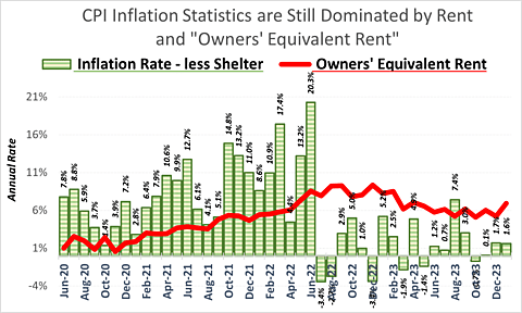
Last May, I wrote a piece called “We Are Measuring Inflation All Wrong: Non‐​housing Inflation Is Very Low.” That has not changed. The uniquely quirky way “shelter” costs are estimated by the US Bureau of Labor Statistics commands such a huge share of the Consumer Price Index (CPI) that it has overwhelmed everything else for nearly two years.

This is mostly due to “Owners’ Equivalent Rent” (OER) which accounts for an astonishing 26.8 percent of the CPI. Rent accounts for another 7.7 percent of the CPI, and hotels for 1 percent.

Owners’ equivalent rent purports to measure monthly variations in a price nobody pays, and to average those estimates for every house in the entire country. Nearly every other country wisely excludes such impossibly arbitrary OER estimates from their measure of inflation. Yet that singular made‐​up number dominates the US CPI, and to a lesser extent the Personal Consumption Expenditures (PCE) inflation index too.

Shelter accounts for 36.1 percent of the CPI and 42 percent of Core CPI. Shelter also accounts for 60 percent of measured inflation in non‐​energy services. This turns out to matter quite a lot, because estimated inflation for shelter has long been extremely high, while inflation for everything else has been extremely low.

The Graph shows that from July 2022 to January 2024, the average CPI inflation rate for shelter was 7 percent, yet the average inflation rate for everything else was only 1.2 percent. This January alone, the reported annual inflation rate for shelter was 6.9 percent, but inflation for everything else was 1.6 percent.

When the January CPI came out, Wall Street Journal reporters Justin Lahart and Nick Timiraos opined that, “Inflation eased again in January but came in above Wall Street’s expectations, clouding the Federal Reserve’s path to rate cuts and potentially giving the central bank breathing space to wait until the middle of the year.” That implied the Federal Open Market Committee might base the next few months’ interest rate manipulations on one month’s “unexpected” OER surge. It also implies that the Fed somehow imagines that keeping the interest rate on bank reserves far above the non‐​housing inflation rate could, in some inexplicable way, diminish future increases in rents.

Federal Reserve apologists prefer to naively accept such official shelter inflation statistics on faith — ostensibly believing that typical market rents have actually been rising at a 7 percent annual rate nationwide— rather than to even consider the possibility that the Bureau of Labor Statistics (BLS) has no idea how to estimate a national average of rents, much less an average of what all houses everywhere might rent for.

We know that is not true because the BLS now collects information about repeat rents for new tenants on the same housing units. The second graph shows that the BLS New Tenant Rent Index was much lower in the fourth quarter of 2023 than it was a year earlier.

If the U.S. measured consumer prices in the same “harmonized” way other countries do —by simply excluding dubious guesstimates of Owners’ Equivalent Rent— the average rate of inflation was 2.3 percent over the past twelve months, 1.1 percent over the past six, and zero over the past three.

Chris Edwards

Policymakers across the nation are concerned about the high costs of housing for moderate‐​income families. One federal response to the problem is the low‐​income housing tax credit (LIHTC), which provides income tax credits to developers of multifamily housing. Currently, Congress is considering expanding the LIHTC and adding a new middle‐​income or workforce version of the credit.

I delivered these comments last Thursday to an American Enterprise Institute conference on the LIHTC. The conference included excellent presentations by Ed Pinto, Tobias Peter, Kevin Corinth, Ed Glaeser, and Howard Husock.

The LIHTC is a complex and inefficient solution to housing affordability. The tax credits crowd out market‐​based housing, benefit financial middlemen more than low‐​income tenants, generate fraud and corruption, and are less efficient than demand‐​side housing aid or free markets. Expanding federal housing tax credits would be the opposite of evidence‐​based policymaking.

Complexity

Governments impose many complex legal structures: income taxation, tax‐​exempt bond rules, environmental rules, building codes, zoning, financial regulations, and dozens of subsidy structures such as Opportunity Zones and community block grants. The LIHTC is complex in itself, and it interacts with all these other complex structures.

How complex is the credit? The bible is the Novogradac 2023 LIHTC Handbook which is 1,798 pages in length. A single tax credit and almost 1,800 pages of rules and guidance!

The federal government apportions housing tax credits to the states, and the states use Qualified Allocation Plans (QAPs) to divvy them out to developers. QAPs are central planning. They micromanage apartment building construction through rules and point systems.

The Virginia QAP and QAP Manual together are 266 pages in length. Some of the complexities include:

Rules for allocating credits to areas within Virginia.
Points for favored neighborhood locations, such as near bus stations.
Points for whether projects have minority and women subcontractors.
Points for developers with experience, giving an advantage to insider firms.
Rules for the financial structure and personnel of developers.
Rules for interactions with other subsidies such as Opportunity Zones.
Points for micromanaging housing unit design. For example, developers receive three points “if each full bathroom’s bath fans are wired to the primary bathroom light with a delayed timer, or continuous exhaust,” three points “if each full bathroom’s bath fans are equipped with a humidistat,” three points if interior doors are solid core, five points for community rooms with certain characteristics, and one point “if each unit has at least one USB charging port in the kitchen, living room, and all bedrooms.”
Rules and points for faucets, shower heads, windows, energy sources, and other green‐​related items.
Rules and points for allowable costs, materials used, accessibility, and many other things.

The Virginia QAP lists 15 types of federal subsidy that LIHTC projects may receive. The Virginia housing agency must do a “Subsidy Layer Review” to ensure that the subsidies fit together within each project. The states must do detailed auditing of LIHTC projects because of fraud problems. There is a layer of federal LIHTC regulations on top of these state QAP rules. The IRS audit guide for the LIHTC is 350 pages in length. All this for one tax credit!

Housing developers need large bureaucracies and face delays in handling all the LIHTC rules. As a result, LIHTC projects cost substantially more to construct than market‐​based projects. Then, after LIHTC projects get built, bureaucracies are needed for long‐​term monitoring of the projects for tenant mix, income levels, and other items for 30 years.

Let me make a political point: Do the nominally conservative Republican members of Congress who support the LIHTC know that it is not a simple investment tax cut, but rather a top‐​down regulatory scheme that imposes massive paperwork burdens on industry and centrally plans homes down to how many USB ports they have?

Corruption

The LIHTC is a vehicle for state and local government corruption, as we have seen in places such as California. In Dallas in 2019, the chair of the housing committee on the city council plead guilty to receiving $40,000 in bribes for trying to steer housing tax credits and other subsidies to a favored developer.

When the federal government gives handouts to state and local governments, it is a fuel for corruption. You see this with many federal programs, such as HUD’s community block grants. One argument against the LIHTC is that the federal government should not be exacerbating the persistent problem of local government corruption with developers.

Tax Reforms for Affordable Housing

I am against special breaks such as the LIHTC, which complicate the tax code. But there are pro‐​market tax reforms that would boost multifamily housing investment.

Reform Tax Depreciation Rules. Apartment buildings have lengthy 27.5‑year depreciation write‐​off periods, which raises effective tax rates on investment. Some apartment building machinery and equipment has shorter depreciation lives that benefited from the 2017 tax bill’s expensing rules, which are now phasing out. Congress should bring back full expensing for machinery and equipment and slash depreciation lives for apartment buildings.
Reduce High Property Taxes. Property taxes on apartment buildings are higher than on owner‐​occupied homes. The Lincoln Land Institute surveys 50 US cities each year, and finds that effective tax rates on apartment buildings are 44 percent higher than on owner‐​occupied homes. That is unfair and undermines multifamily investment. Cities should cut property taxes on apartment buildings.

Regulations Raise Costs and Reduce Innovation

Rather than micromanage multifamily development with the LIHTC, we need innovation in low‐​cost housing production such as modular construction, tiny houses, and new materials. Regulations are the enemy of such innovations.

In a 2022 study, the trade associations NAHB and NMHC found that regulations raise costs of apartment building construction by 41 percent. Higher costs stem from constant changes to building codes, affordability mandates, land set‐​asides, government delays, labor regulations, complex zoning approvals, unique development mandates, and developer fees. On top of that 41 percent regulatory cost, the study found that NIMBY battles add another 6 percent to development costs.

The study was based on a survey of multifamily developers. Half the developers said they would not build in places with inclusionary zoning mandates and 88 percent said they would not build in places with rent controls. The report concludes that “regulatory mandates discourage developers from building in the very marketplaces that have the greatest need for more housing.” Government solutions often backfire.

The Terner Center for Housing Innovation at Berkeley studies the costs of LIHTC projects. The center found that in 2019 prevailing wage laws in California increased the average cost of building LIHTC projects from about $400,000 per unit to about $500,000. LIHTC projects are high‐​cost construction.

Here is a final point on regulation. Economic studies, such as a 2022 NBER study by Goolsbee and Syverson, note that construction industry productivity has been stagnant for decades. While total factor productivity has trended upward in the overall economy, productivity in construction has dipped since the 1970s. Economists do not know exactly why, but overregulation that stifles innovation is one likely cause. We are building homes roughly the same way we did 50 years ago. Manufactured products are far cheaper today than in the past, but home construction is more expensive. The low‐​income housing tax credit compounds this regulatory cost problem.

To conclude, the way ahead should be deregulation, innovation, and lower costs, not more subsidies, higher costs, and central planning with tax‐​credit programs.

The LIHTC is explored by Chris Edwards and Vanessa Calder in this study.

Jai Kedia

Capital One recently announced plans to acquire Discover Financial Services with a $35.3 billion all‐​shares transaction. The proposed merger has brought the usual suspects out of the political woodwork to complain about financial concentration and increasing bank size.

For instance, Senate Banking Committee Chair Sherrod Brown (D‑OH) complained that a deal that “makes powerful financial companies even bigger and more powerful will do nothing for families.” Sen. Elizabeth Warren (D‑MA) echoed similar sentiments, saying the deal “threatens our financial stability, reduces competition, and would increase fees and credit costs for American families.”

Unsurprisingly, these critics who levy concerns about the size and power of private financial institutions show little concern about the balance sheet of the Federal Reserve—whose assets have grown exponentially since the financial crisis.

As of Q4 2023, Capital One and Discover reported total assets of $478.5 and $151.5 billion respectively (collectively about $630 billion). Their combined balance sheet represents less than 3 percent of the total assets held by commercial banks in the US. In the same quarter, the Fed reported average asset holdings of $7.8 trillion—over one‐​third the size of the entire US commercial banking sector. It is also double the $3.9 trillion in assets held by Chase, the largest bank in the US.

More troubling is the trend of the Fed’s increases in balance sheet size. Figure 1 shows the size of the Fed’s balance sheet in proportion to all US commercial banks. Prior to the 2008 financial crisis, the Fed’s balance sheet rarely exceeded 10 percent of the commercial banking sector, with the trend exhibiting a gentle decline. Since the financial crisis, the Fed entered a new era with this number frequently exceeding 20 percent. Since Covid‐​19, the Fed now holds so many assets that it is well over 30 percent, the size of all commercial banking.

To be fair, the Fed does attempt to reduce its balance sheet size following a massive surge. However, as Covid‐​19 demonstrated, if it is now expected to buy assets following every major economic shock, there is no way it will ever revert to a pre‐​financial crisis state.

Unlike private institutions, whose balance sheet increases do not harm the macroeconomy, the Fed purchases vast quantities of US treasuries to facilitate the government’s spending spree. Given the massive effects such fiscal expansion has on inflation and the role it played in the post‐​Covid price surge, Congress would do well to rein in the Fed’s balance sheet instead of debating mergers between private financial institutions.

The author thanks Jerome Famularo for providing research assistance during the preparation of this essay. All data used in this analysis was collected from the FRED website.